[1] "2026-05-20"2 Start Here: Workflow, Quarto, And RStudio
2.1 Learning Goals
By the end of this chapter, the main goals are:
- open and navigate the course project
- understand the relationship among R, RStudio, Posit Cloud, and Quarto
- run code chunks inside a
.qmdfile - render a Quarto document to HTML
- use source mode, visual mode, and the document outline intentionally
2.2 The Course Workflow
This course uses R for computation, RStudio for the working interface, and Quarto for the documents that combine prose, code, and output. The goal is not only to make individual plots. The goal is to build a reproducible workflow where the text explains the question, the code performs the work, and the output records what happened.
During class, most work will happen inside .qmd files like this one. A Quarto file is a plain-text document that can contain headings, paragraphs, lists, links, code chunks, tables, figures, and notes about interpretation. When Quarto renders the file, it runs the code chunks and combines the results with the surrounding text.
This is different from working only in the console. The console is useful for quick tests, but it does not automatically preserve the reasoning around the command. A Quarto document keeps the analysis in order: what question was being asked, what data were used, what code was run, what output appeared, and what conclusion followed.
2.3 Literate Programming
Donald Knuth — who wrote The Art of Computer Programming and built the TeX typesetting system — coined the term literate programming in 1984. The idea is to write code primarily for human readers rather than for computers. Explanation and code go in the same document, in the same order as the reasoning, so a reader can follow both at once.
Most statistical work has not been done this way. The standard workflow for a long time has been: run the analysis in Stata or R, save the plots and tables to a folder somewhere, open Word, write the paper, load the figures in, open PowerPoint, build the slides, load the figures in again. Get a comment from a co-author, go back to Stata, re-run something, save a new version of the figure, find all the places it appears in Word and PowerPoint, replace them. Repeat. The analysis and the document are separate objects that have to be kept in sync by hand.
This works, after a fashion, but it is slow, it is error-prone, and it makes replication hard. A table in the slides may not match the one in the paper. A figure may have been made with an earlier cut of the data. Six months later, you may not be able to reconstruct exactly which version of the code produced a given number.
Quarto solves this by putting everything in one place. The prose, the code, the figures, and the tables all live in a single .qmd file. Render it and you get a paper, a slide deck, or a report — whatever the YAML specifies. Change the data or revise the analysis, render again, and all the outputs update at once. Nothing is pasted in from elsewhere and nothing gets out of sync.
It is worth saying something about LaTeX here, because it has been the standard for scientific publishing for decades, and for good reason. LaTeX produces beautiful output. The typesetting is precise, the mathematical notation is unmatched, and the journal templates for economics, political science, sociology, psychology, statistics, and most other quantitative disciplines are built for it. Many journals still expect it.
The problem is that LaTeX is genuinely hard to use and remarkably unforgiving. One missing brace and the document fails to compile with an error message that tells you very little. The syntax is arcane. Managing bibliographies, cross-references, and figure placement requires learning a small universe of packages. Collaborating on a LaTeX document means everyone needs a working installation and the patience to debug it. This is not like Word, where you type, save, and look at what you have.
Quarto gives you most of what LaTeX offers without requiring you to write it directly. Quarto uses Markdown as its writing format — plain text with simple conventions for headings, bold, lists, and links — and is the successor to R Markdown, which many researchers in these fields will have encountered. R Markdown established the idea of mixing R code with prose in a single document; Quarto takes that further, adding support for Python and other languages, a more consistent syntax, and better tools for books, websites, and presentations. When you render a .qmd file to PDF, Quarto calls LaTeX under the hood — so the output looks like a LaTeX document, journal templates work, and equations render properly — but you write in Markdown. You get the output quality without the brittleness. When you need to go further into LaTeX directly, it is there, but for most purposes you will not need to.
The tidyverse extends this thinking down to the code itself. Hadley Wickham designed dplyr and ggplot2 to be read as well as run. A pipeline written with |> reads left to right: take this data, filter it, reshape it, summarize it by group. A ggplot2 call names explicitly what each variable does in the plot and why. The code is not just instructions for R — it is a record of the decisions made during the analysis, which is exactly what Knuth had in mind.
The Examples/Party Rolls folder shows this in a real project, covered in more detail later in this chapter.
2.4 Plain R Scripts
The simplest kind of R source file is a plain R script. A plain R script uses the .R extension and contains only R code. It is useful for setup tasks, repeated checks, helper functions, and other code that does not need surrounding prose or rendered output.
This project includes a few plain R scripts:
install_packages.R
check_setup.R
The file check_setup.R is a good example. It checks whether the course packages and course data files are available. Opening that file and clicking Source runs the whole script. The result is a quick setup check, not a rendered document.
Use .R scripts when the goal is to run code directly. Use .qmd files when the goal is to combine explanation, code, and output.
2.5 The Console
The console is the fastest place to test a command, inspect an object, or rerun something without rendering a document.
Two console habits are especially helpful:
- the up arrow cycles through recent commands
Ctrl + Rsearches command history in many RStudio setups
The console is not a replacement for a source file. If a command becomes part of the analysis, move it into a .qmd or .R file so it is preserved.
2.6 R, RStudio, Posit Cloud, And Quarto
These tools have different jobs:
- R is the programming language that reads data, transforms it, estimates models, and makes graphics.
- RStudio is the interface where you edit files, run code, inspect objects, view plots, and render documents.
- Posit Cloud is a browser-based version of the RStudio workflow that avoids many local installation problems.
- Quarto is the publishing system that turns
.qmdsource files into HTML, PDF, Word, slides, dashboards, and books.
R Markdown was the predecessor used in earlier versions of this course. Quarto keeps the same basic idea, but it is now the preferred format for this version of the workshop. If you have used .Rmd files before, the transition should feel familiar: a .qmd file still mixes text and code. The main difference is that Quarto uses a more general and consistent document system.
2.7 Project Files And Portable Paths
The examples in this course assume that the project has been opened in RStudio or Posit Cloud. Files are organized inside the project in folders such as Data/, Demos/, and Exercises/.
The data examples use file names like these:
Data/gapminder/gapminder.csv
Data/penguins/penguins.csv
Demos/presentation-demo.qmd
Exercises/04-scatterplot-solution.R
Avoid file names that depend on a personal Desktop, Downloads folder, or another location on one person’s computer.
Keeping files inside the project matters because the course should work in Posit Cloud, on another computer, or after being archived for later use.
2.8 The RStudio Layout
RStudio usually has four main panes:
- the source pane, where
.qmdand.Rfiles are edited - the console, where commands can be typed and run directly
- the environment and history pane, where current objects and previous commands are listed
- the files, plots, packages, help, and viewer pane
The exact pane arrangement can be changed under Global Options. The important habit is to know which pane is doing which job. The source pane is for durable work. The console is for quick tests. The environment pane shows what objects currently exist. The viewer pane is often where rendered HTML output appears.
2.9 RStudio Settings
A few RStudio settings can make workshop work more comfortable:
- turn off restoring
.RDatainto the workspace at startup - set saving the workspace on exit to “Never”
- turn on rainbow parentheses if available
- use the document outline for long
.qmdfiles - choose a source editor font and size that are comfortable for several hours of reading
These settings do not change the analysis, but they reduce friction. The main principle is that the project files should define the work, not a hidden workspace image from a previous session.
2.10 Source Mode And Visual Mode
RStudio can edit Quarto documents in source mode or visual mode.
Source mode shows the underlying Markdown and code exactly as written. It is the most transparent mode for learning because it makes headings, chunks, chunk options, links, and lists visible.
Visual mode is a more word-processor-like interface. It can be helpful for editing prose, tables, footnotes, and links. It is still editing the same .qmd file, but it hides some of the raw syntax while you write.
Both modes are useful. During this course, source mode is usually the clearest mode for understanding how the document works. Visual mode can be helpful later when revising narrative text.
2.11 Markdown Basics
Quarto uses Markdown for ordinary text formatting. A few patterns cover most needs:
# First-level heading

## Second-level heading

Regular paragraph text.

- a bullet point
- another bullet point

**bold text**

*italic text*

[Quarto website](https://quarto.org)
The number of # symbols controls the heading level. Headings also create the document outline, which makes long lessons easier to navigate.
2.12 Code Chunks
An R code chunk starts with three backticks and {r}. A useful chunk also has a short name after r, then ends with three backticks.
In the source file, the opening line would be ```{r ch02-code-chunks-1} and the closing line would be ```. The R code between those lines could be:
1 + 1The code inside the chunk can be run interactively, and it can also be run during rendering. In RStudio, you can run a chunk with the green play button or with keyboard shortcuts. You can insert a new chunk from the menu or by typing the chunk delimiters yourself.
If that chunk runs, the result would be:
[1] 2Chunks can contain more than one line. For example:
x <- 10
y <- 25
x + y
The assignment operator <- stores a value in an object. In the example above, x stores 10 and y stores 25. After those objects exist, R can use them in later commands.
2.14 Chunk Options
Chunk options control how code behaves during rendering. In Quarto, options are often written as special comment lines at the top of the chunk.
This chunk runs but hides the code:
This chunk displays code without running it:
Sys.Date()eval: false is important for examples that require credentials, internet access, private files, or intentional manual action. The code remains visible as a template, but it does not run automatically.
2.15 Rendering
Rendering turns a source .qmd file into an output document. For this course, HTML is the primary output because it is easy to view in a browser and works well for code, figures, tables, and links.
When you render a document, Quarto starts from the top, runs the chunks in order, and inserts the output where it belongs. If a chunk fails, rendering stops. That is useful because it exposes broken code early.
The render button in RStudio is the easiest way to start. Open the file and click Render to create the output document. PDF output is also useful for papers, handouts, and print-ready reports, but it depends on a working TeX installation. Posit Cloud’s tidyverse template already has TeX installed, so PDF rendering works without any additional setup. On a local machine without TeX, the tinytex package provides a lightweight installation:
install.packages("tinytex")
tinytex::install_tinytex()
2.16 A Real Workflow: From Presentation to Published Paper
The Examples/Party Rolls folder shows this in practice. The files trace one research project from early results to publication:
rolls23.Rmd— a presentation written in R Markdown. Rendering it producesrolls23.pdf, a slide deck.agenda_leviathan23.Rmd— the manuscript version of the same project, with different formatting and tables. Rendering it producesagenda_leviathan23.pdf, the submitted manuscript.shor and kistner 2023.pdf— the final published version, typeset by the journal.
The presentation and the manuscript share the same underlying code. When the analysis changed, it changed in one place and both outputs updated.
2.17 Output Formats
Quarto can produce many output formats from the same source file:
- HTML documents and books
- PDF reports
- Word documents
- RevealJS slides
- dashboards
- websites
2.17.1 Presentation Demo
A presentation file uses a revealjs format in the YAML header. Second-level headings become slides.
---
title: "Presentation Demo"
format:
  revealjs:
    theme: simple
---
## Slide Title
Slide text goes here.The course includes a standalone demo at Demos/presentation-demo.qmd. Code chunks work the same way as in a chapter, but slides usually hide the code and show the output.
2.17.2 Paper Or Report Demo
A paper-style document adds a bibliography file and uses article as the document class. Citations use keys from the .bib file.
---
title: "Paper Demo"
author: "Name"
bibliography: paper-example.bib
format:
  html: default
  pdf: default
---
The course includes Demos/paper-example.qmd and Demos/paper-example.bib. Citations are written as [@wickham_ggplot2_2016].
2.18 A First Reproducible Example
The built-in mtcars dataset is available in base R, so it is useful for a first test that does not depend on course data files.
head(mtcars)This command creates a simple base R plot:
plot(mtcars$wt, mtcars$mpg)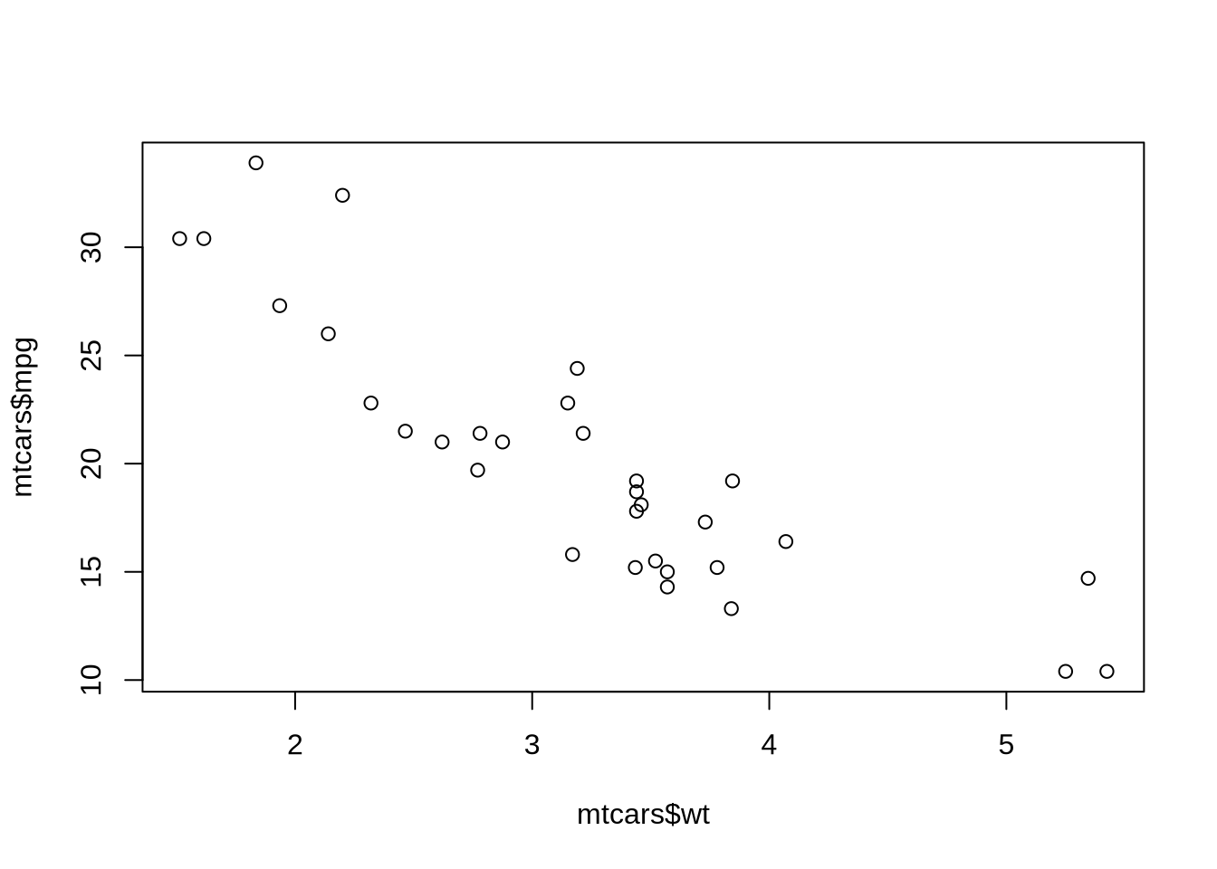
The plot is not polished, but it confirms that R is running, code chunks are executing, and graphical output appears in the document.
2.19 Reading Output Carefully
A rendered document is not automatically correct just because it renders. Rendering answers one question: did the code run from top to bottom? You still have to ask whether the data are the right data, whether the variables mean what you think they mean, whether missing values were handled correctly, and whether the plot supports the claim being made.
This course will return to that distinction throughout the week. Reproducibility is necessary, but it is not enough. A reproducible mistake is still a mistake.
2.20 Short Exercise
Create a new code chunk below this paragraph. In that chunk:
- store the number
100in an object namedstart_value - store the number
25in an object namedchange_value - subtract
change_valuefromstart_value
# Write your code here.2.21 What Comes Next
The next chapter begins the data workflow: importing files, inspecting tibbles, reshaping data, and using the core tidyverse verbs that prepare data for visualization.